4.Filtering in the frequency domain

4.1 Background

4.1.1 A Brief history of the Fourier series and transform

- Fourier series or transform can be reconstructed completely via an inverse process with no loss of information

4.1.2 About the example

-More effective tool and filtering technique than Chapter 3’s smoothing and sharpening

4.2 Preliminary concepts

4.2.1 Complex Numbers

	-A complex number C is defined as C = R + jI  ( * j is imaginary number)  ㅡ>   ( Conjugate of a complex number) C* = R - jI 
	ㅡ> C = |C|(cos θ + j sinθ)  (Complex number in polar coordinates) ㅡ> (Using Euler’s formula) C = |C|e^jθ

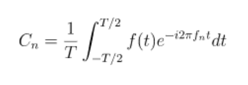
4.2.2 Fourier Series

4.2.3 Impulses and their sifting property

-Central to the study of linear systems and the Fourier transform is the concept of an impulse and its sifting property
-Periodic impulses can be continuous or discrete

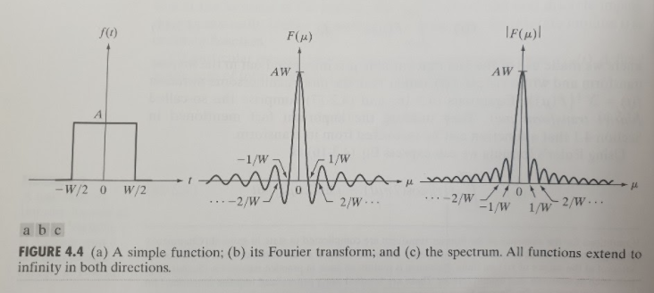
4.2.4 The Fourier Transform of functions of One continuous

4.2.5 Convolution -We can obtain the convolution in the spatial domain by computing the inverse Fourier transform -Convolution theorem is that the expression on the right is obtained by Fourier transform, and the foundation of filtering in the frequency domain

4.3 Sampling and the Fourier transform of sampled functions

4.3.1 The sampling theorem -Continuous function have to be converted into a sequence of discrete values before they can be processed in a computer. -This is accomplished by using sampling and quantization

4.3.2 The Fourier transform of sampled functions

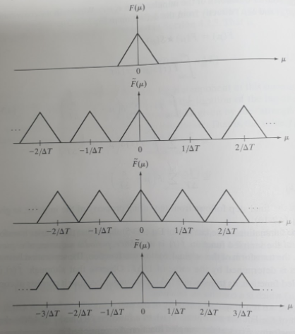
-(a) is a sketch of the Fourier transform
-(b) is results of an over-sampled signal
-(c) is the results of critically- sampling
-(d) is the results of under-sampling

4.3.3 The sampling theorem -The sampling theorem is the result of equation that continuous, band-limited function can be recovered completely from a set of its samples

4.3.4 Aliasing -Aliasing is a process in which high frequency components of a continuous function “masquerade” as lower frequencies in the sampled function -This is consistent with the common use of the term alias , which means “ a false identity”

4.3.5 Function Reconstruction from sampled data -The reconstruction of a function reduces in practice to linear interpolating between the samples

4.6 Some Properties of the 2-D Discrete Fourier Transform

4.6.1 Relationships Between Spatial and Frequency Intervals -They are Inverse proportional

4.6.2 Translation and Rotation -Rotating by same angle

4.6.3 Periodicity -As in the 1-D case , the 2-D Fourier transform and its inverse are infinitely periodic

4.6.4 Symmetry Properties -Because all indices in the DFT and IDFT are positive, Functions are said to be symmetric and odd functions are antisymmetric

4.6.5 Fourier Spectrum and Phase angle -If the phase was set to zero , there is no shape information in the image

4.6.6 The 2-D Convolution Theorem -DFT algorithms tend to execute faster with arrays of even size

4.6.7 Summary of 2-D Discrete Fourier Transform Properties -Formula

4.8 Image smoothing using frequency domain filters

4.8.1 Ideal Lowpass filters -The blurring and ringing properties of ILPFs can be explained using the convolution theorem

4.8.2 Butterworth Lowpass filter - Unlike the ILPF, the BLPE transfer function does not have a sharp discontinuity

4.8.3 Gaussian Lowpass filter -The profile of the GLPF is not as “tight” as the profile of the BLPF. It is an important characteristic in practice in medical imaging

4.8.4 Additional examples of lowpass filtering -Lowpass filtering is a staple in the printing and publishing industry

4.9 Image sharpening using frequency domain filters

4.9.1 Ideal Highpass filters -Highpass filtering is analogous to differentiation in the spatial domain

4.9.2 Butterworth Highpass filters -The transition into higher values of cutoff frequencies is much smoother with the BHPF

4.9.3 Gaussian Highpass filters -The filtering of the smaller objects and thin bars is cleaner with the Gaussian filter

4.9.4 The Laplacian in the frequency domain -It has the same scaling issues just mentioned, compounded by the fact

4.9.5 Unsharp masking, highboost filtering, and high frequency emphasis filtering -The result obtained using a combination of high frequency emphasis and histogram equalization is superior to the result

4.9.6 Homomorphic filtering -This filter is similar to the high emphasis filter discussed in the previous section