1.Data Mining(2)

5.Data Preprocessing

• 5.1 Aggregation
• Combining two or more attributes (or objects) into a single attribute (or object)
• Purpose
  • Data reduction
    • Reduce the number of attributes or objects
  • Change of scale
    • Cities aggregated into regions, states, countries, etc.
    • Days aggregated into weeks, months, or years
  • More “stable” data
    • Aggregated data tends to have less variability
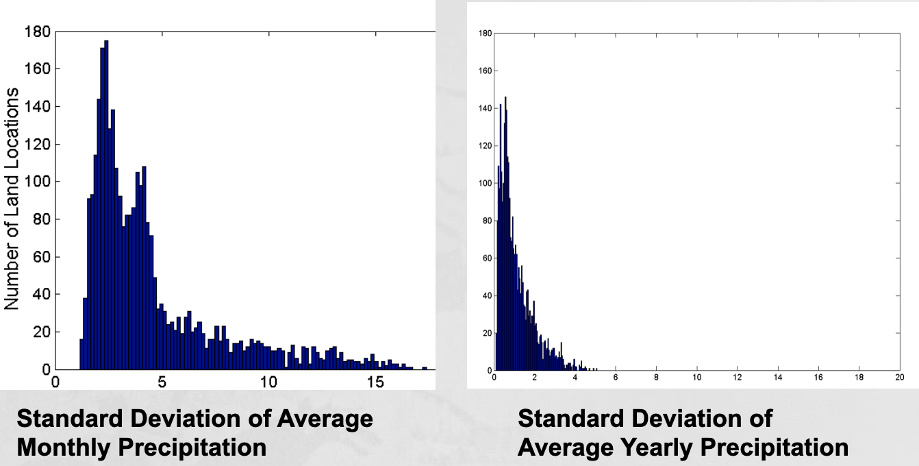
• Example: Precipitation in Australia
  • This example is based on precipitation in Australia from the period 1982 to 1993.
  • The next slide shows
    • A histogram for the standard deviation of average monthly precipitation for 3,030 0.5◦ by 0.5◦ grid cells in Australia, and
    • A histogram for the standard deviation of the average yearly precipitation for the same locations.
  • The average yearly precipitation has less variability than the average monthly precipitation.
  • All precipitation measurements (and their standard deviations) are in centimeters.

• 5.2 Sampling
  • Sampling is the main technique employed for data reduction.
    • It is often used for both the preliminary investigation of the data and the final data analysis.

  • Statisticians often sample because obtaining the entire set of data of interest is too expensive or time consuming.

  • Sampling is typically used in data mining because processing the entire set of data of interest is too expensive or time consuming.

  • The key principle for effective sampling is the following:

    • Using a sample will work almost as well as using the entire data set, if the sample is representative
    • A sample is representative if it has approximately the same properties (of interest) as the original set of data

• Types of Sampling
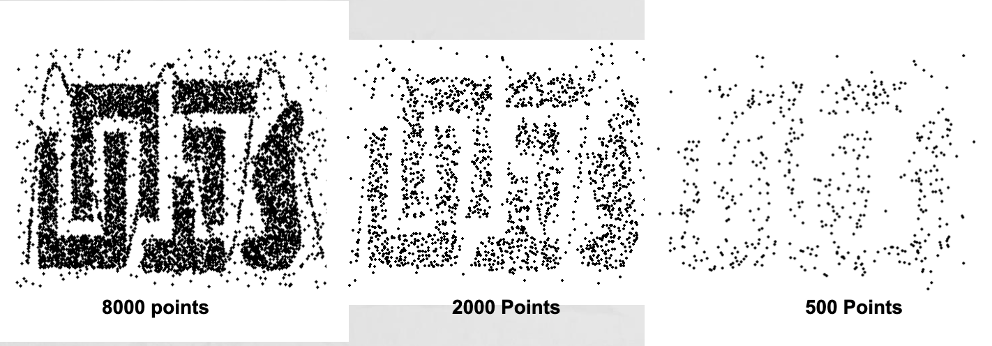
  • Simple Random Sampling
    • There is an equal probability of selecting any particular item
    • Sampling without replacement
      • As each item is selected, it is removed from the population
    • Sampling with replacement
      • Objects are not removed from the population as they are selected for the sample.
      • In sampling with replacement, the same object can be picked up more than once
    • Stratified sampling
      • Split the data into several partitions; then draw random samples from each partition

• 5.3 Dimensionality Reduction

• Purpose:
  • Avoid curse of dimensionality
  • Reduce amount of time and memory required by data mining algorithms
  • Allow data to be more easily visualized
  • May help to eliminate irrelevant features or reduce noise
• Techniques
  • Principal Components Analysis (PCA)
  • Singular Value Decomposition
  • Others: supervised and non-linear techniques
• Curse of Dimensionality

  • When dimensionality increases, data becomes increasingly sparse in the space that it occupies

  • Definitions of density and distance between points, which are critical for clustering and outlier detection, become less meaningful

• Dimensionality Reduction: PCA

  • Goal is to find a projection that captures the largest amount of variation in data

• 5.4 Feature subset selection

• Another way to reduce dimensionality of data
• Redundant features
  • Duplicate much or all of the information contained in one or more other attributes
  • Example: purchase price of a product and the amount of sales tax paid
• Irrelevant features
  • Contain no information that is useful for the data mining task at hand
  • Example: students’ ID is often irrelevant to the task of predicting students’ GPA

• Many techniques developed, especially for classification

• 5.6 Feature creation

• Feature creation

  • Create new attributes that can capture the important information in a data set much more efficiently than the original attributes

  • Three general methodologies:
    • Feature extraction
      • Example: extracting edges from images
  • Feature construction - Example: dividing mass by volume to get density
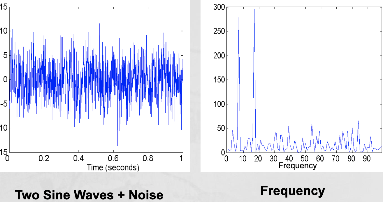
  • Mapping data to new space - Example: Fourier and wavelet analysis

• 5.7 Discretization and Binarization

• Discretization is the process of converting a continuous attribute into an ordinal attribute
  • A potentially infinite number of values are mapped into a small number of categories
  • Discretization is commonly used in classification
  • Many classification algorithms work best if both the independent and dependent variables have only a few values
  • We give an illustration of the usefulness of discretization using the Iris data set
• Binarization

  • Binarization maps a continuous or categorical attribute into one or more binary variables

  • Typically used for association analysis

  • Often convert a continuous attribute to a categorical attribute and then convert a categorical attribute to a set of binary attributes

    • Association analysis needs asymmetric binary attributes
    • Examples: eye color and height measured as 
{low, medium, high}

• 5.8 Attribute Transformation

• An attribute transform is a function that maps the entire set of values of a given attribute to a new set of replacement values such that each old value can be identified with one of the new values

  • Simple functions: xk, log(x), ex,

    x

  • Normalization
    • Refers to various techniques to adjust to differences among attributes in terms of frequency of occurrence, mean, variance, range
    • Take out unwanted, common signal, e.g., seasonality
  • In statistics, standardization refers to subtracting off the means and dividing by the standard deviation