1.Data Mining

1.Attributes and Objects

• What is Data?

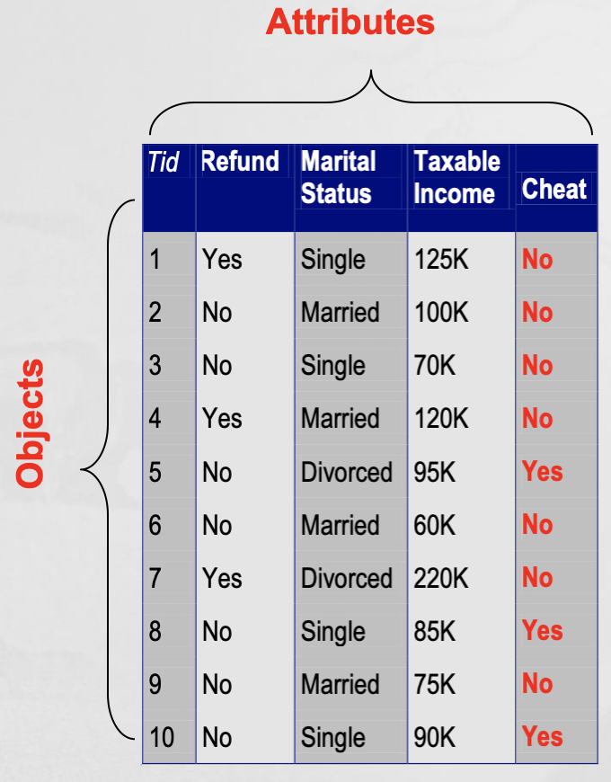
• Collection of data objects and their attributes

• An attribute is a property or characteristic of an object
  • Example : eye color of a person, temperature, etc.
  • Attribute is also known as variable, field, characteristc, dimension, or feature
  • A collection of attributes describe an object
    • Object is also known as record, point, case, sample, entity, or instance
• A more Complete View of data
  • Data may have parts
  • Attibutes (objects) may have relationships with other attirbutes (objects)
  • More generally, data may have structure
  • Data can be incomplete
  • We will discuss this in more dtail later
• Attribute Values
  • Attribute values are numbers or symbols assigned to an attribute for a particular object
  • Distinction between attributes and attribute values
    • Same attribute can be mapped to different attribute values
      • Example: height can be measured in feet or meters
  • Different attributes can be mapped to the same set of values
    • Example: Attribute values for ID and age are integers
    • But properties of attribute values can be different

2.Types of Data

• 데이터 셋은 객체로 구성된다
  • entity, 레코드, 점, 벡터, 패턴, 사건, 사례, 표본, 케스 등의 명칭 사용
• 객체는 물리적 객체의 질량이나 사건이 일어난 시간과 같이 주어진 객체의 기본적 특성을 표현하는 다수의 속성에 의해서 기술된다
  • 변수, 특성, 특징, 차원, 필드

• attribute 먼저, 그 다음 object 순서로..

• Tpyes of attributes
  • There are different types of attributes
    • Nominal
      • Ex : ID numbers, eye color, zip code
    • Ordinal
      • Ex : rankings (e.g, taste of potato chips on a scale from 1-10), grades, height(tall,medium,short)
    • Interval
      • Ex : calendar dates, temperatures in Celsius or Fahrenheit
    • Ratio
      • Ex : temperature in Kelvin, length, counts, elapsed time (e.g., time to run a race)
• Properties of Attribute Values
  • Distinctness : = ≠
  • Order : < >
  • Differences are meaningful : + -
  • Ratios are meaningful : * /

  
  

  • Nominal attribute: distinctness
  • Ordinal attribute: distinctness & order
  • Interval attribute: distinctness, order & meaningful differences
  • Ratio attribute: all 4 properties/operations
• Difference Between Ratio and Interval
  • Is it physically meaningful to say that a temperature of 10 ° is twice that of 5° on
    • the Celsius scale?
    • the Fahrenheit scale?
    • the Kelvin scale?
  • Consider measuring the height above average
    • If Bill’s height is three inches above average and Bob’s height is six inches above average, then would we say that Bob is twice as tall as Bill?
    • Is this situation analogous to that of temperature?
• Categorization of attributes is due to S.S. Stevens
  • Categorical Quantitative
    • Nominal : Nominal attibute values only distinguish (=,≠) (e.g., zip code, employee ID numbers, eye color) , (Operations : mode enthropy, contingency corrlation)
    • Ordinal : Ordinal attibute values also order object (<,>) (e.g., hardness of minerals, grades, street numbers) , (Operation : median, percentiles, rank corrlation, run tests, sign tests)
  • Numeric Quantitative
    • Interval : For interval attributes, differences between values are meaningful (+,-) (e.g., calendar dates, temperature in Celsius or Fahrenheit) , (Operation : mean, standard deviation, Pearson’s correlation)
    • Ratio : For ratio variables, both differences and ratios are meaningful (*,/) (e.g., temperature in Kelvin, monetary quantities, counts,age, mass, length, current) , (Operations : geometric mean, harmonic mean, percent variation)
  • Categorical Quantitative
    • Nominal : Any permutation of values (Comments : If all employee ID numbers were reassigned, would it make any difference?)
    • Ordinal : An order preserving change of values (Comments : An attribute encompassing the notion of good, better best can be represented equally well by the values {1,2,3} or by {0.5 , 1, 10})
  • Numeric Quantitative
    • Interval : new_value = a * old_value + b where a and b are constants (Comments : Thus, the Fahrenheit and Celsius temperature scales differ in terms of where their zero value is and the size of a unit)
    • Ratio : new_value = a * old_value (Length can be measured in meters of feet)
• Discrete and Continuous Attirbutes
  • Discrete Attribute
    • Has only a finite or countably infinite set of values
    • Examples: zip codes, counts, or the set of words in a collection of documents
    • Often represented as integer variables.
    • Note: binary attributes are a special case of discrete attributes
  • Continuous Attribute
    • Has real numbers as attribute values
    • Examples: temperature, height, or weight.
    • Practically, real values can only be measured and represented using a finite number of digits.
    • Continuous attributes are typically represented as floating-point variables.

• Asymmetric Attiributes

  • Only presence (a non-zero attribute value) is regarded as important
    • Words present in documents
    • Items present in customer transactions

  • If we met a friend in the grocery store would we ever say the following? “I see our purchases are very similar since we didn’t buy most of the same things.”

  • We need two asymmetric binary attributes to represent one ordinary binary attribute
    • Association analysis uses asymmetric attributes
  • Asymmetric attributes typically arise from objects that are sets

• Key Messages for Attribute Types

  • The types of operations you choose should be “meaningful” for the type of data you have

    • Distinctness, order, meaningful intervals, and meaningful ratios are only four properties of data

    • The data type you see – often numbers or strings – may not capture all the properties or may suggest properties that are not present

    • Analysis may depend on these other properties of the data

    • Many statistical analyses depend only on the distribution

    • Many times what is meaningful is measured by statistical significance

    • But in the end, what is meaningful is measured by the domain

2.3 Types of data sets

• Type
  • Record
    • Data Matrix
    • Document Data
    • Transaction Data
  • Graph
    • World Wide Web
    • Molecular Structures
  • Ordered
    • Spatial Data
    • Temporal Data
    • Sequential Data
    • Genetic Sequence Data

• Important Charateristics of Data
  • Dimensionality (number of attributes)
    • High dimensional data brings a number of challenges
  • Sparsity
    • Only presence counts
  • Resolution
    • Patterns depend on the scale
  • Size
    • Type of analysis may depend on size of data
• Record Data
  • Data that consists of a collection of records, each of which consists of a fixed set of attributes

• Data matrix

  • If data objects have the same fixed set of numeric attributes, then the data objects can be thought of as points in a multi-dimensional space, where each dimension represents a distinct attribute

  • Such a data set can be represented by an m by n matrix, where there are m rows, one for each object, and n columns, one for each attribute

• Document Data
  • Each document becomes a ‘term’ vector
  • Each term is a component (attribute) of the vector
  • The value of each component is the number of times the corresponding term occurs in the document
• Transaction Data
  • A special type of data, where
    • Each transaction involves a set of items.
    • For example, consider a grocery store. The set of products purchased by a customer during one shopping trip constitute a transaction, while the individual products that were purchased are the items.
    • Can represent transaction data as record data
• Graph Data
  • Examples: Generic graph, a molecule, and webpages
• Ordered Data
  • Sequential transactions
  • Genomic sequence data
  • Spatial - Temporal Data

3.Data Quality

• Data Quality

  • Poor data quality negatively affects many data processing efforts “The most important point is that poor data quality is an unfolding disaster.
    • Poor data quality costs the typical company at least ten percent (10%) of revenue; twenty percent (20%) is probably a better estimate.” Thomas C. Redman, DM Review, August 2004
  • Data mining example: a classification model for detecting people who are loan risks is built using poor data
    • Some credit-worthy candidates are denied loans
    • More loans are given to individuals that default

• Measurement and Data Collection Issues

  • What kinds of data quality problems?
  • How can we detect problems with the data?
  • What can we do about these problems?
  • Examples of data quality problems:
    • Noise and outliers
    • Missing values
    • Duplicate data
    • Wrong data
    • Fake data
• Noise
  • For objects, noise is an extraneous object
  • For attributes, noise refers to modification of original values
    • Examples: distortion of a person’s voice when talking on a poor phone and “snow” on television screen
• Outliers
  • Outliers are data objects with characteristics that are considerably different than most of the other data objects in the data set
    • Case 1: Outliers are noise that interfereswith data analysis
    • Case 2: Outliers are the goal of our analysis
      • Credit card fraud
      • Intrusion detection
• Missing Values
  • Reasons for missing values
    • Information is not collected (e.g., people decline to give their age and weight)
    • Attributes may not be applicable to all cases (e.g., annual income is not applicable to children)
  • Handling missing values
    • Eliminate data objects or variables
    • Estimate missing values
      • Example: time series of temperature
      • Example: census results
    • Ignore the missing value during analysis
  • Missing completely at random (MCAR)
    • Missingness of a value is independent of attributes
    • Fill in values based on the attribute
    • Analysis may be unbiased overall
  • Missing at Random (MAR)
    • Missingness is related to other variables
    • Fill in values based other values
    • Almost always produces a bias in the analysis
  • Missing Not at Random (MNAR)
    • Missingness is related to unobserved measurements
    • Informative or non-ignorable missingness
  • Not possible to know the situation from the data
• Duplicate Data
  • Data set may include data objects that are duplicates, or almost duplicates of one another
    • Major issue when merging data from heterogeneous sources
  • Examples:
    • Same person with multiple email addresses
  • Data cleaning
    • Process of dealing with duplicate data issues
  • When should duplicate data not be removed?

4. Similarity and Distance (유사도)

• Similarity and Dissimilarity Measures
  • Similarity measure
    • Numerical measure of how alike two data objects are.
    • Is higher when objects are more alike.
    • Often falls in the range [0,1]
  • Dissimilarity measure
    • Numerical measure of how different two data objects are
    • Lower when objects are more alike
    • Minimum dissimilarity is often 0
    • Upper limit varies
  • Proximity refers to a similarity or dissimilarity

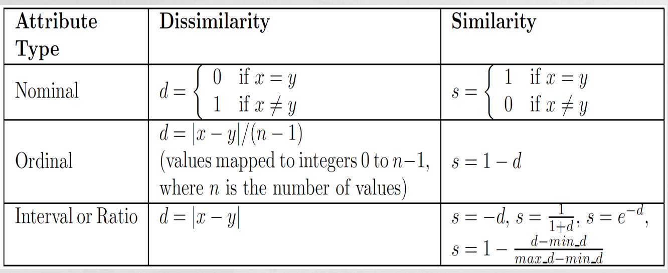
• Similarity/Dissimilarity for Simple Attributes

  • The following table shows the similarity and dissimilarity between two objects, x and y, with respect to a single, simple attribute.

• Dissimilarities between Data Objects
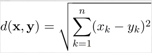
  • Euclidean Distance

  

  • where n is the number of dimensions (attributes) and xk and yk are, respectively, the kth attributes (components) or data objects x and y

  • Minkowski Distance

  

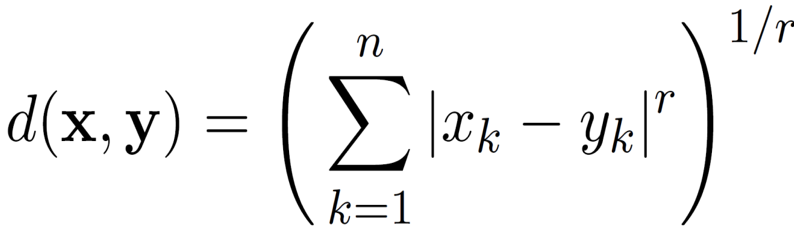
  • r = 1. City block (Manhattan, taxicab, L1 norm) distance.
    • A common example of this for binary vectors is the Hamming distance, which is just the number of bits that are different between two binary vectors

  • r = 2. Euclidean distance

  • r → ∞. “supremum” (Lmax norm, L∞ norm) distance.
    • This is the maximum difference between any component of the vectors
  • Do not confuse r with n, i.e., all these distances are defined for all numbers of dimensions.

• Similarity

  • Similarities, also have some well known properties.

    • s(x, y) = 1 (or maximum similarity) only if x = y. (does not always hold, e.g., cosine)
    • s(x, y) = s(y, x) for all x and y. (Symmetry)
      • where s(x, y) is the similarity between points (data objects), x and y.

• Similarity Between Binary Vectors

  • Common situation is that objects, x and y, have only binary attributes

  • Compute similarities using the following quantities f01 = the number of attributes where x was 0 and y was 1 f10 = the number of attributes where x was 1 and y was 0 f00 = the number of attributes where x was 0 and y was 0 f11 = the number of attributes where x was 1 and y was 1

  • Simple Matching and Jaccard Coefficients SMC = number of matches / number of attributes = (f11 + f00) / (f01 + f10 + f11 + f00)

    J = number of 11 matches / number of non-zero attributes = (f11) / (f01 + f10 + f11)

• Cosine Similarity

  • If d1 and d2 are two document vectors, then cos( d1, d2 ) = <d1,d2> / ||d1|| ||d2|| ,

  • where <d1,d2> indicates inner product or vector dot product of vectors, d1 and d2, and

    d

    is the length of vector d.

  • Example: d1 = 3 2 0 5 0 0 0 2 0 0 d2 = 1 0 0 0 0 0 0 1 0 2

<d1, d2> = 31 + 20 + 00 + 50 + 00 + 00 + 00 + 21 + 00 + 02 = 5

d1

= (33+22+00+55+00+00+00+22+00+00)0.5 = (42) 0.5 = 6.481

d2

= (11+00+00+00+00+00+00+11+00+22) 0.5 = (6) 0.5 = 2.449

cos(d1, d2 ) = 0.3150

• Correlation

  • Correlation measures the linear relationship between objects

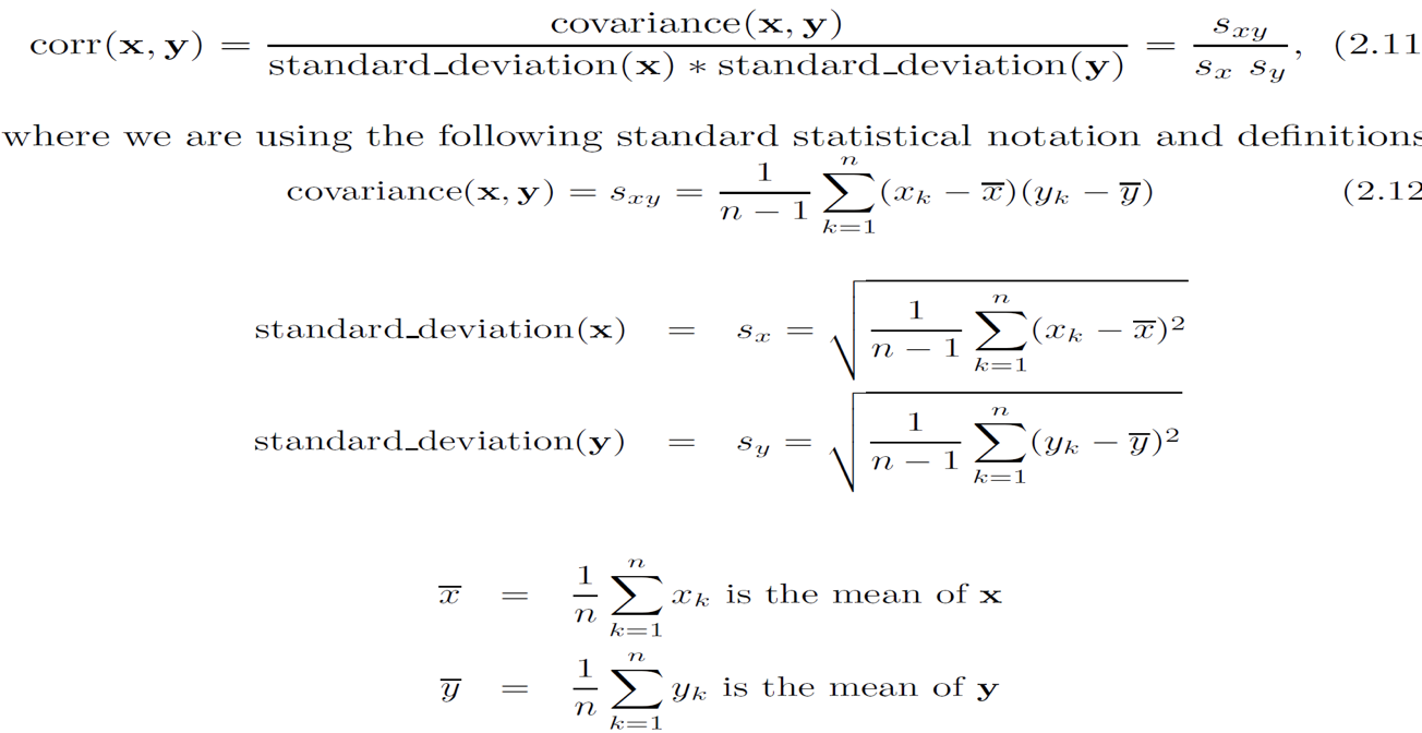
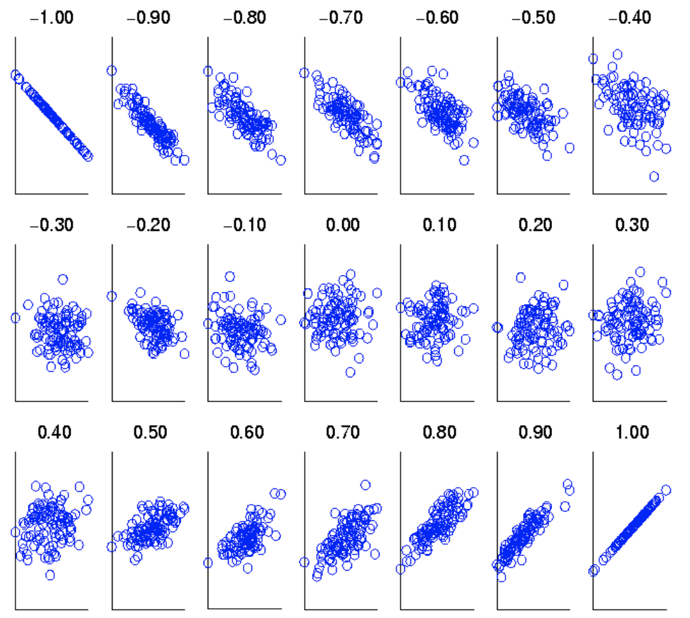
- Visually Evaluating Correlation

• Comparison of Proximity Measures

  • Domain of application
    • Similarity measures tend to be specific to the type of attribute and data
      • Record data, images, graphs, sequences, 3D-protein structure, etc. tend to have different measures
  • However, one can talk about various properties that you would like a proximity measure to have
    • Symmetry is a common one
    • Tolerance to noise and outliers is another
    • Ability to find more types of patterns?
    • Many others possible
  • The measure must be applicable to the data and produce results that agree with domain knowledge

• Combining Similarities

  • General Approach for Combining Similarities
    • Sometimes attributes are of many different types, but an overall similarity is needed.
    • 1: For the kth attribute, compute a similarity, sk(x, y), in the range [0, 1].
    • 2: Define an indicator variable, δk, for the kth attribute as follows:
      • δk = 0 if the kth attribute is an asymmetric attribute and both objects have a value of 0, or if one of the objects has a missing value for the kth attribute
    • δk = 1 otherwise

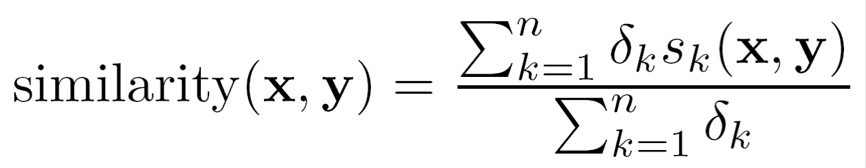
    - Using Weights to Combine Similarities
    - May not want to treat all attributes the same.

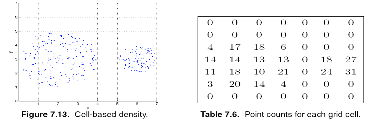
• Density
  • Measures the degree to which data objects are close to each other in a specified area
  • The notion of density is closely related to that of proximity
  • Concept of density is typically used for clustering and anomaly detection
  • Examples:
    • Euclidean density
      • Euclidean density = number of points per unit volume
    • Probability density
      • Estimate what the distribution of the data looks like
    • Graph-based density
      • Connectivity
• Euclidean Density: Grid-based Approach Simplest approach is to divide region into a number of rectangular cells of equal volume and define density as # of points the cell contains

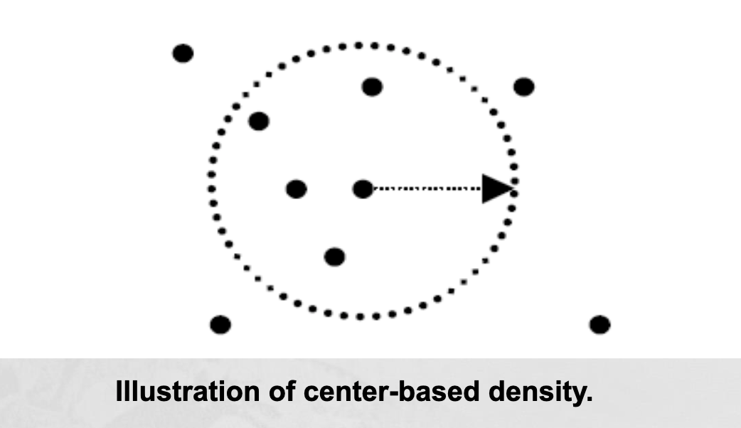
• Euclidean Density: Center-Based Euclidean density is the number of points within a specified radius of the point